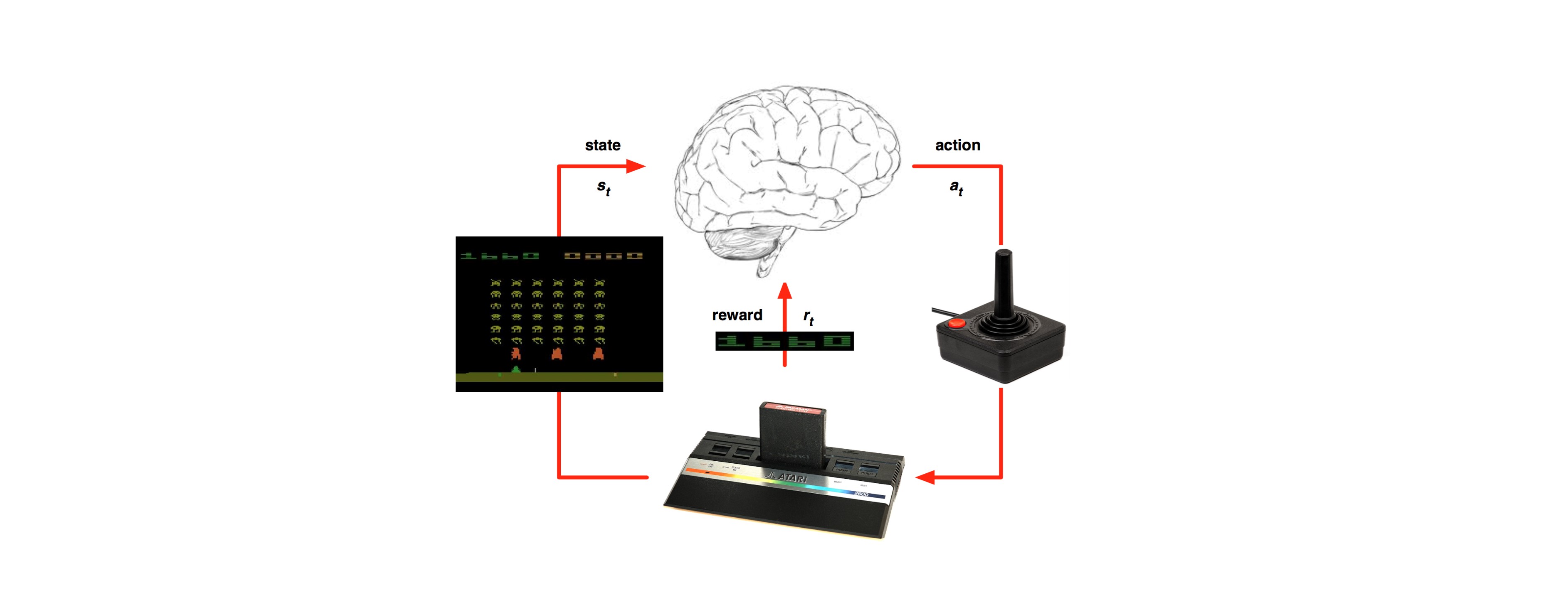
In the previous part we’ve learned about the standard formulation setting of RL (MDP): https://g-stat.com/reinforcement-learning-series-getting-the-basics-part-2. This article would be about a basic method in RL – Monte-Carlo (MC). As stated in the previous part MDP needs information about the environment, but MC is model free i.e. it only uses the experience, tuples of state, action and reward, gained by the agent.

Monte-Carlo uses random samplings, in order to get a numerical estimation. We use MC methods in RL to get the average sample returns for each state. We sample multiple sequences of states action pairs from starting state to the terminal state, each sample is called an “episode”.  The episodes are used to estimate the future reward gained from using a certain policy in the subsequent states.

In MC two steps are used iteratively to get the optimal policy – evaluation and policy improvement. We start with evaluating a certain policy, afterwards bettering it and repeat:

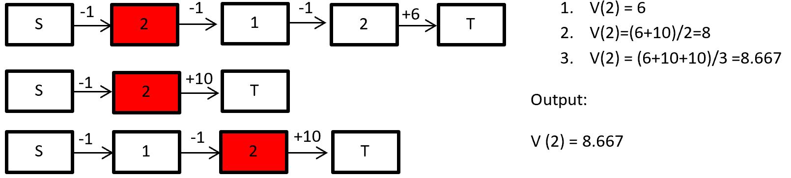
During the evaluation step we learn the value functions for a certain policy via empirical mean of the cumulative future discounted reward. There are two ways of creating a mean: “First Visit” and “Every Visit”. In first visit we take all the first time steps that state s is visited and average their returns. For example if we want to calculate the state-value function for state 2:

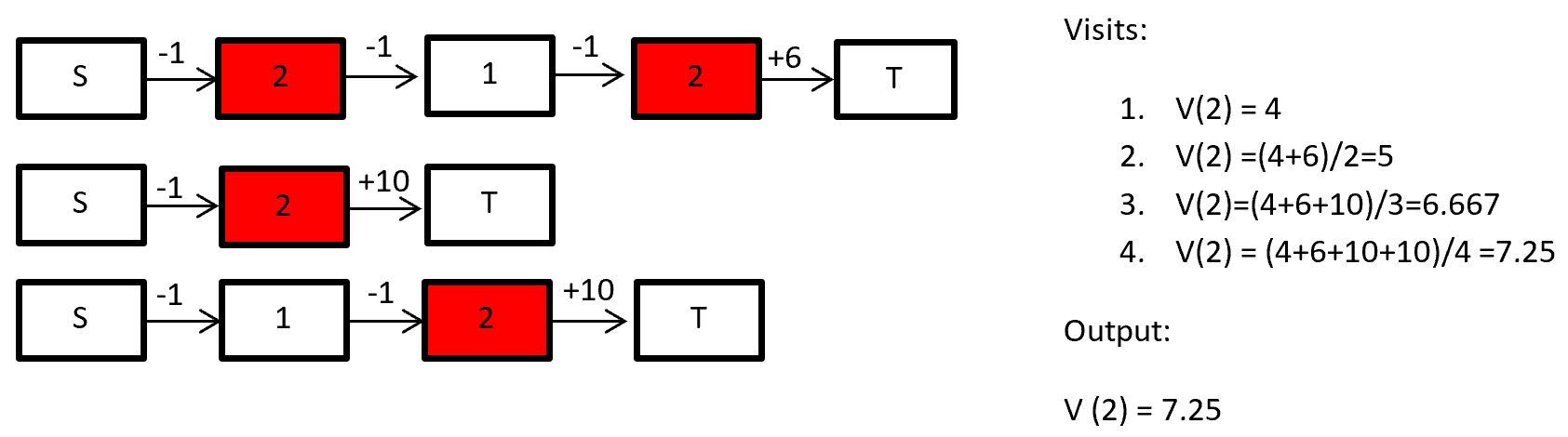
In every visit we take every time step that state s is visited and average their returns. For example if we want to calculate the state-value function for state 2:

It’s also possible calculating the action-value function, if we average pairs of state and action.

In the policy improvement step we change the policy in order to get a better one.  A “better” policy is a new policy that has greater values for at least one state, while the other states’ values are equal to the previous policy. The first solution that comes to mind is bettering the policy greedily, but as expected we would usually end up in a local optimum.  We want to converge on the optimal actions. There’s a theorem proves that convergence can be gained by using “Greedy in the limit of Infinite Exploration” (GLIE) optimization methods. GLIE methods are basically methods that theoretically converge on a greedy policy while all the state-action pairs are explored infinite times.

The most common GLIE method is  – greedy.  In – greedy the policy for a certain state is to pick at random with the probability, otherwise we pick an action greedily with probability 1 –. The is decaying along the run, thus, making it GLIE. We might make some bad actions, but sometimes we need to explore different places in the state space to find the optimal solution.

The -greedy method allows us using the hyper-parameter  in order to balance the trade-off between exploration and exploitation. On one side we want to explore, thus, we want high and low decaying rate, but on the other hand we want to exploit the knowledge gained, thus, we want low and high decaying rate. There are multiple ways of picking the right hyper parameters of a problem, such as grid search, evolutionary methods and other state space search methods. So choose a method of your liking and see how your agent acts. Would he be able to get first place in Mario Kart with a certain? Or will it get the last?

The main advantage from MC is that we learn from complete episodes, thus, not introducing extra bias. On the other side the variance of returns can be high, and it can only be used on tasks that terminates.

In the next part we will learn about “Temporal difference”, a method that tries to solve MC’s disadvantages.