Last time we’ve talked about learning from partial episodes with the TD methodology: https://g-stat.com/reinforcement-learning-series-getting-the-basics-part-4/. Another issue that rises while solving RL problems – what should we do with problems that are too big like Go (
The methods that help representing and estimating the functions in these problems are called value function approximation. In this article we would only review value function approximation via deep neural network; moreover, we would see how to implement it in a popular methodology called Deep Q-Network (DQN). DQN is a methodology developed by DeepMind in 2013. It was used to beat human experts in multiple Atari games. DQN solves problems that use picture frames as states but can be modified for continuous problems. I would use the hyper parameters of the DQN paper but remember that they might need some tweaking to best suit your own problem.

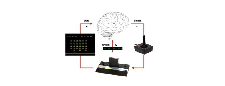
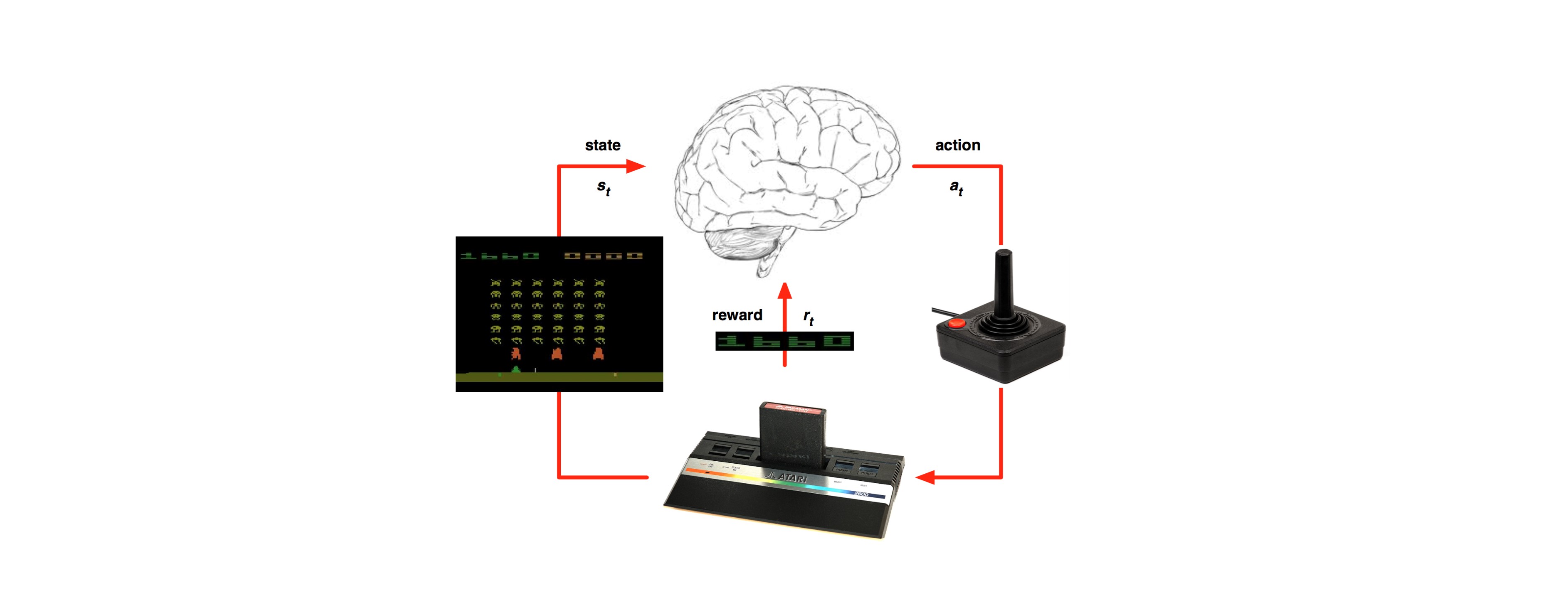
Figure 1 Atari's Space Invaders – one of the games DQN beat human experts
As we’ve learned in the first article there are differences between RL and supervised learning. As we all know DNN is a supervised learning method that requires the input to be i.i.d. Otherwise, the model might be overfitted for some samples and the solution wouldn’t be generalized. Moreover, in Q learning we want to predict the action value function, but after certain time steps we are updating it. This way we’ve got labels that change over time for the same input. This stability condition for the output and input is needed for the DNN to perform well. However, in RL both input and the target change constantly during the learning process making the training process to be unstable. This unstable learning process is basically like a dog chasing his own tail.
We’ve already seen the input and output can converge. So we might have a chance to model the action value function while allowing it to evolve, if we slow down the changes in the input and output. In DQN we accomplish this in two ways:
Experience replay – Using a buffer in which we would put 1,000,000 transitions and sample a mini batch of 32 transitions from this buffer to train the DNN (the buffer and the mini batch sizes are hyper parameters). This way we stabilize the input, because random samplings from the replay buffer are more independent, thus making the mini batch closer to I.I.D. As we create new transition, we would replace old transitions with new ones.
Target network – Creating two DNN
DQN uses Huber loss instead of quadratic loss we are used to have in supervised learning. Huber loss has quadratic values while in range of a certain
The DNN architecture takes 4 sequential pictures frames and feed it to convolution layer that at the end computes the action values for each action for the input state (4 sequential pictures):

For your convenience I’ve added the pseudo code from DeepMind’s article:
Deep Q-learning with experience replay |
Initialize replay memory D to capacity N Initialize action-value function Q with random weights Initialize target action-value function For episode = 1 to M do: Initialize sequence For t= 1 to T do: With probability Otherwise select Execute action Set Store transition ( Sample random minibatch of transitions ( Set Perform a gradient decent step on Parameters Every C steps rest End for End for
*
https://arxiv.org/pdf/1312.5602.pdf |
This is the last part of the series I hope you’ve learned a lot and that I’ve ignited a desire within you to use and study RL even more. If you want to dig deeper, I recommend reading Sutton’s and Barto’s “Reinforcement Learning an Introduction” or watch David Silver’s lectures on YouTube.
Yours truly, Don Shaked