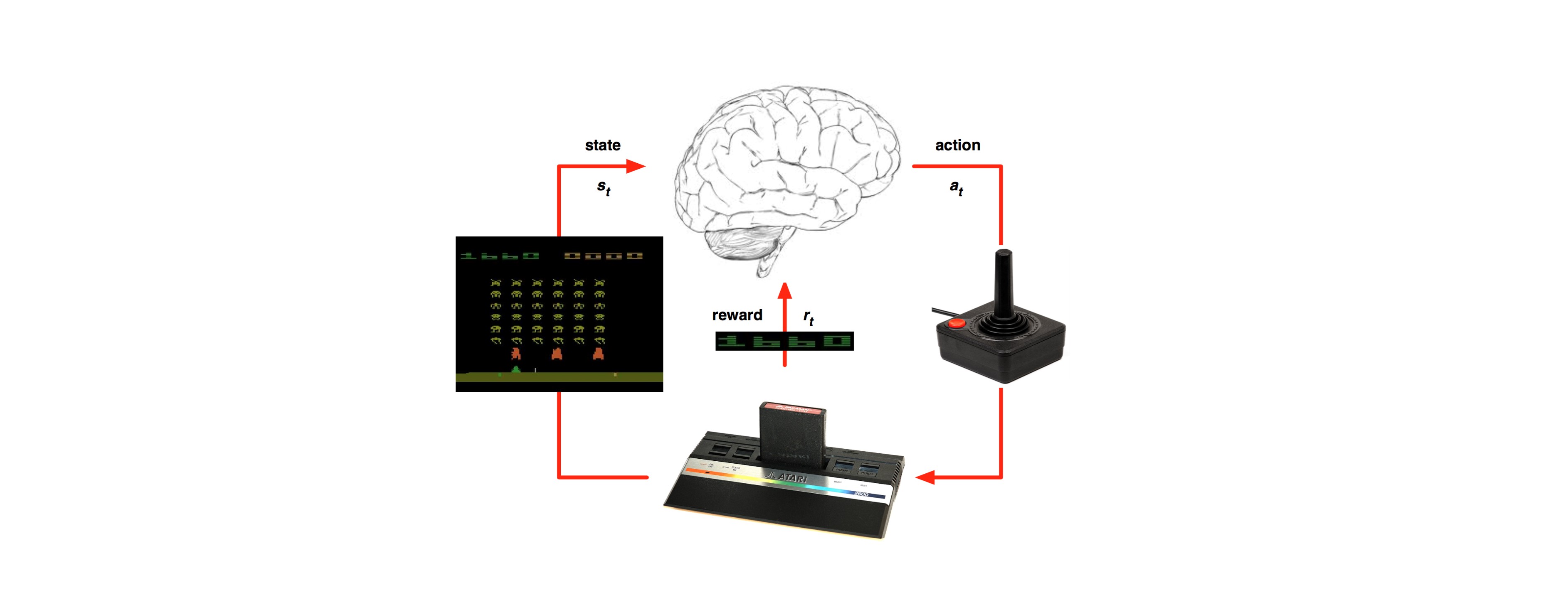
Last time we’ve tipped our feet in the water and got some understanding of the basic terminology of the RL world: https://g-stat.com/reinforcement-learning-getting-the-basics-series/. In this article we would learn about Markov Decision Process (MDP), which is the formulation setting for almost all RL problems.

MDP is a discrete time control modelling process, the process may be stochastic or deterministic. The major property of MDPs is independency of the future to the past given the present i.e. the present state contains all the information needed to value the future. This property is known as the Markov property, and it can always be true because we can define the state as all the history. Using all the history creates a huge state space and usually it’s a terrible idea.  For example in the grid world a state would be the cell we are in, and the history representation would be all the cells we’ve been until this point.

In order to solve the MDP problem it’s needed to define 2 new definitions:

Action value function – The value function of taking action a in state s under a policy , denoted , is the expected return when starting in s, taking action a, and following  thereafter. We can write the Action value function using the Bellman equations as:

Where  is the reward given from doing action a in s,  is the discount factor,  is the probability of moving from state s to s’ using action a,  is the probability of using new action a’ in new state s’ and  is the Action value function of the next state s’ given a’.

State value function – The value function of a state s under a policy , denoted , is the expected return when starting in s and following  thereafter (The value of a terminal state is always zero).  We can write the State value function using the Bellman equations as:

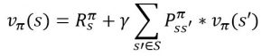
Where  is the reward given from using policy in state s,  is the probability of moving from state s to s’ using policy  and  is the State value function of the next state.

From this definition we understand that it’s possible to calculate the state value function from the action value function and not vice versa, because . Calculating the value of each state value function and action value function given a policy is an easy task solving linear equations and known as Markov Reward Process (MRP).  We will need to solve |S| equations for the state value function and |A|*|S| equations for the action value function.

The problem is that usually we don’t know which policy is the best policy; finding the best policy means optimizing the MDP problem. We usually optimize MDP with dynamic programing method such as policy iteration. In general we are starting from a certain policy evaluating it and better the solution in a greedy fashion. Going greedy in the current setting will get us the optimal solution (proved in policy improvement theorem). The concept of evaluation and then improvement is a reoccurring element in RL.

As explained before MDP is a discrete time control modelling process in which all the knowledge about the environment is known.  There are many expansions for this model adjusting it for different cases. The major ones are: continuity of the state or action space, continuous time and missing information about the environment. That can be solved via linear quadratic model, Hamilton-Jacobi Bellman (HJB) differential equations, and partially observed MDP (POMDP) respectively.

Even though we are using MDP as the formulation setting there are big differences between MDP and RL. Opposing to MDP we don’t use any information of the environment, only the experiences (states, actions and rewards of each time step) thus making the environment a black box. Moreover the reward is sampled without knowing the underlying model of neither the reward function nor the state transition probabilities. The lack of knowledge usage makes the performance of RL weaker to other methods which take advantage of the knowledge. In the paper of Guo at al, NIPS 2014 they compered the scores of a trained DQN (one of the  RL methods we will learn in this series) to the scores of a standard off the shelf Monte Carlo tree search and received better results :

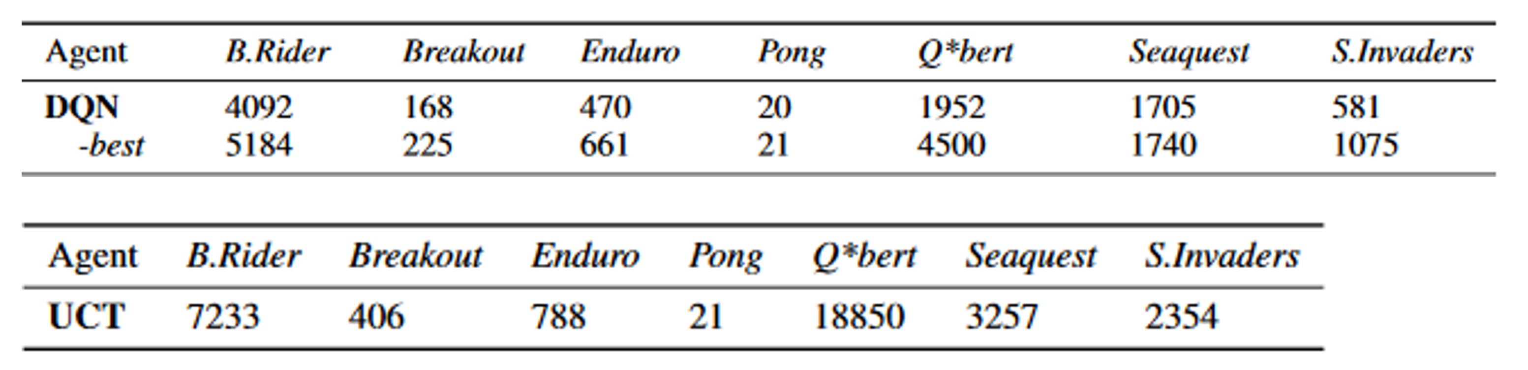
The big “but” is that the DQN learned everything from RAW pixels without tuning for each game individually, you didn’t need to be an expert of the “black box”. To quote Bruce Lee “You must be shapeless, formless, like water. When you pour water in a cup, it becomes the cup. When you pour water in a bottle, it becomes the bottle… Water can drip and it can crash. Become like water my friend.” RL in that sense is like water, the methods of RL are general and fit easily to the problem we want to solve. 

Next time we will learn about different RL methods.