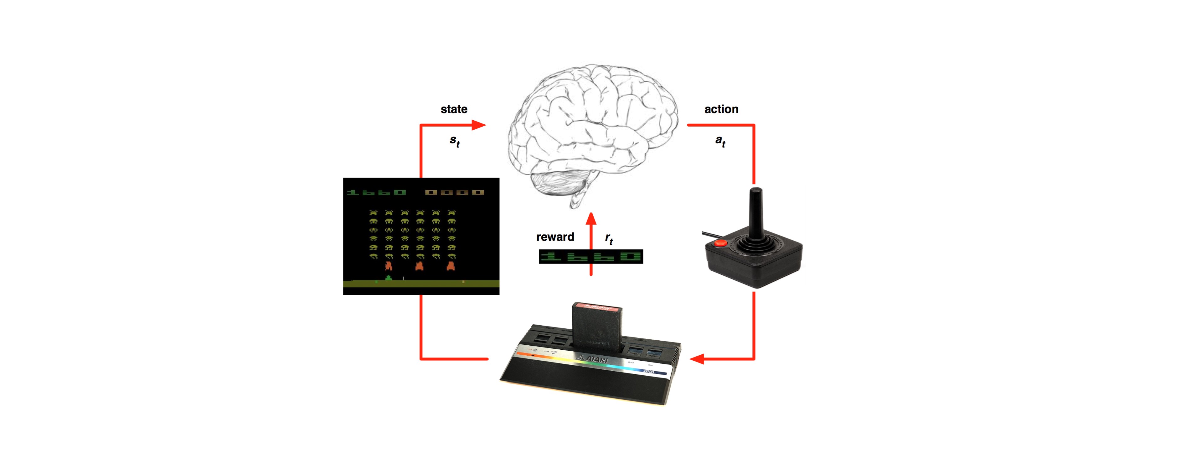
Last time we’ve learned about the Monte Carole methodology in RL: https://g-stat.com/reinforcement-learning-series-getting-the-basics-part-3/. As mentioned MC can only be used on the whole episode, thus, limiting us to learn only when the episode terminates. In order to solve this problem we want to learn from partial episodes – the “go-to” methodology in RL that can do it is called Temporal Difference (TD).
TD methods doesn’t have to wait until the end of the episode to determine the change of the value functions, they only have to wait until the next time step. At the next time step these methods can form an estimator and make a useful update using the observed reward and the estimate of the next state’s state value function [V(V(St+1))]. In this article we would learn about 2 TD methods: TD (0) and TD (λ). Moreover we would see how to use policy improvement for TD.
TD (0) is the simplest TD method. As discussed in the previous article; MC updates the values according to the accumulated discounted reward from the terminal state. Whereas TD (0) updates the value functions immediately on transition i.e. after receiving the next state and reward. We update the value function in this manner:
VSt←VSt+α(Rt+1+γVSt+1-V(St))
Where α∈(0,1]
TD (λ) is basically using exponential discounting on all viewed history, where λ is the discounting factor. The last terminal state gets the reminder of the weights, this way the steps’ weights sums up to 1. When λ equals to zero, we are putting all the weight on one step ahead and we would get TD (0). When λ equals to one, we are putting all the weight on the last step and we would get MC. The exponential discounting is done in the following way:

There are two implementations of TD (λ): forward and backward view. The forward view is a theoretical view of exponential discounting over n-step future returns. In this article we would focus on backward view, but it has been proven that both forward and backward views are equivalent. The backward view updates values at each step. After each step in the episode you make updates to all prior steps by using Eligibility Traces (ET). ET is a record of the frequency of entering a certain state and defined as:
E0s=0
Et+1s=λ Ets+1St=s
Where λ is a discount factors for the frequency of the state.
We will update the value function by using the ET on the delta between the old observation and the new one this way:
δt=Rt+1+γVSt+1-V(St)
V(s)=V(s)+αδtEts
Both MC and TD converge to the real values for #episode→∞. MC has high variance and zero bias. This is because the return depends on many random actions, transitions and rewards, yet the return is unbiased (the true return of that state). TD has low variance and some bias. This is because TD depends on doesn’t only use the true return or doesn’t use the true return at all (TD (0)). If we want to get the best of both worlds we can use the TD (λ) that can be used to mitigate between variance and bias. However we will have to search λ as any other hyper parameter we’ve got.
As we can see the methods above are used for estimating a certain policy. Usually when we are at the policy improvement stage we would rather use the action value function (QSt), this is because we would gain a better understanding of a better policy. In order to get the best policy we can use the ε greedy method we’ve met in the last article. We can either make the adjustments offline (after an episode terminated) or online (during an episode). If we do the policy improvement offline we will go over all the states and update them according to ε greedy. If we do the policy improvement online we would choose the best action from our current understanding at each new state we are facing. We can either do it on the observed value – SARSA, or on the estimated value – Q-learning. For your use I’ve added pseudo code for SARSA and Q-learning using TD (0) evaluation:

A note about the initialization, if you have prior knowledge about the states you can use it in the initialization, thus accelerating the convergence of the RL algorithm.
Next time we will learn how to use value function approximation.

