Reinforcement learning (RL) is a rising field in the Machine learning (ML) scene. in this article we will understand what is RL, what problems we can solve with RL and how we formulate the RL problem. This article is the first of a series of articles that will cover the RL field at an introductory level.
RL is the process of learning how to map actions to states in order to maximize a numerical reward signal. The learner isn’t told what to do but rather to discover which actions yield the most accumulated reward by trying them and estimating the accumulated reward from the observed scenarios (bootstrapping). The actions in a RL problem may affect not only the immediate reward but also future reward. This means that the data in the RL problem isn’t I.I.D (independent and identically distributed) which is a major difference to other fields in ML (supervised/unsupervised).
Usually the RL problem is formulated as an optimal control of Markov decision process (MDP). This idea captures the most important aspects of the RL problem. There’s an agent (or the learner) selects actions and the environment is responding these actions with a reward and presenting the agent a new situation.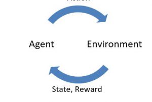
The MDP is defined by:
1.States (S) – states can be discrete like my place in a grid world
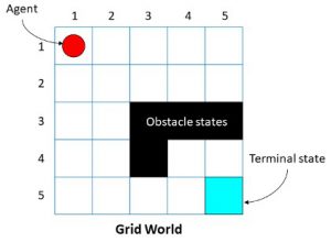
Figure 1 Matlab's Grid world
The state is the bracket in which the agent is at.
The states can be continuous like a data we are getting from sensor about a robot’s joint angles, velocity and distance from the target.
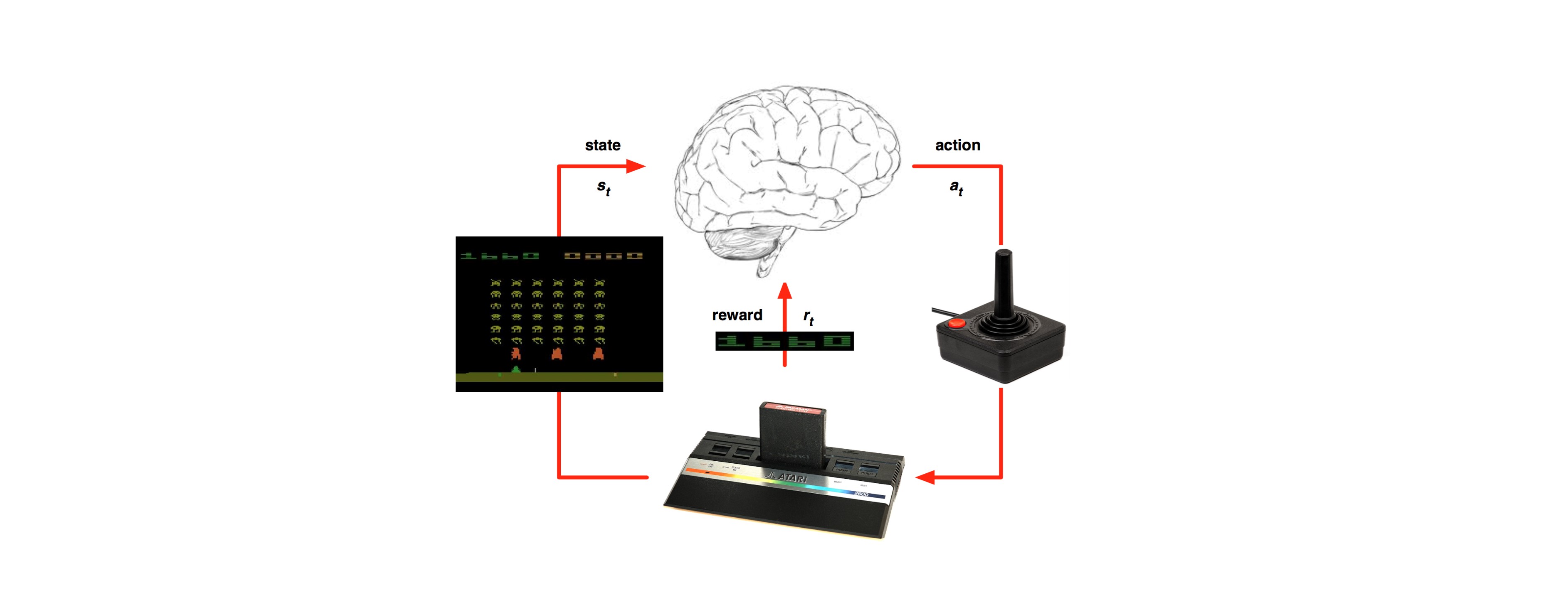
The states can be even represented by an image:

Figure 2 Atari's Space Invaders
This can be represented as a state via CNN.
2. Starting state (So) – the state in which the agent starts can be random or constant.
3. Actions (A(s)) – what can the agent do in a certain state? In the first example there are 4 possible moves (moving north, east, west or south); in the second example the action we can do is change the speed of a certain joint; in the Atari example we can go left/right and shoot. Here we can see that even an action can be either discrete or continuous.
4. Reward function(R(s, a, s’)) – numerical signal we get from the environment after doing an action (a) in a certain state (s) and moving to a new state (s’). Some environments already encapsulate a good representation of a reward but if you want to create a new environment let’s say an autonomous car we need to think for what we need to give the reward. For example we want to reach the target place as fast as we can so we might give a reward for driving in a high velocity but we also want to avoid pedestrian so want to give a negative reward for getting near them and so on.
5. Discount factor (γ) – discount factor is meant to discount future rewards just like bankers do with money i.e. money in the future has smaller current value. The main use of discount factor is that the solutions would convergence better.
6. Transition function (P(s’|s, a)) – sometime we have the probability to move to a new state (s’) after we’ve taken action (a) in state (s). Problems that have a transition matrix also called a Model of the environment. If the environment doesn’t have a transition matrix the environment will be called Model-free.
![]()
7. Policy – what action should we do in a certain state? A policy can be deterministic or stochastic. In the grid world example a deterministic policy is always going north and a stochastic policy is going north for 50% and south 50%.
Even though there are big differences between RL and supervised learning there were tries to solving RL problems via supervised learning, this is called “imitation learning”. In this approach the machine is learning to choose the right action to do in each stage which is represented by feature and the data set is solved cases by experts. The biggest issue with this approach is that it cannot recover from failures; a good example of this could be that the expert never got himself to this situation. This is the problem of compounding error, in fact there’s a lower bound to the supervised
imitation learning error (Kääriäinen, 2006) which is essentially), where ![]() is the number of sequential decision and the error of the prediction.
is the number of sequential decision and the error of the prediction.